Hey! I'm David, cofounder of zkSecurity and the author of the Real-World Cryptography book. I was previously a crypto architect at O(1) Labs (working on the Mina cryptocurrency), before that I was the security lead for Diem (formerly Libra) at Novi (Facebook), and a security consultant for the Cryptography Services of NCC Group. This is my blog about cryptography and security and other related topics that I find interesting.
Years ago, naive me lost a lot of money because he was too stingy to hire a financial advisor, and too lazy to do some basic research. Hopefully you don't make the same mistakes. It took me a while to post this because, I didn't know if I should, I didn't understand the trouble I was in really, and I felt really dumb at the time.
Disclaimer: if you are in this situation don't just trust me, do your own research and hire your own financial advisor.
It all started when some of my coworkers at Facebook warned me that when the financial year came to an end, they realized that they still owed dozens of thousands of dollars in taxes. This might sound like an outrageous number, but one might think that it's also OK as "if you earn more it's normal to pay more taxes". Years later, when this happened to me, I realized that I could almost have ended up in debt.
Let me explain: stocks or tokens that you receive as payment is paper money, but not for the IRS. For the government it's worth as much as the "fair market value" of that stock or token at the moment your employer sends it to you. For the government, it's like income in USD, so they'll still tax you on that even if you haven't converted these in USD yourself.
Let me give you an example: your company has a token that's worth 1,000,000 USD. They send you 1 token, which the IRS will see as an event of you receiving one million dollars of income. In that moment, if you don't sell, or if you're too slow to sell, and the price drops to 1 USD, you're still going to owe the IRS one million dollars.
What's tricky is that even if you decide to sell the stock/token directly, its fair market value (however you decide to calculate it) can be highly uncorrelated to the price you sell it at. That's because tokens are known to be fairly volatile, and (if you're lucky) especially during the time it takes to receive and then sell it.
If that's not enough, you also pay taxes (called capital gain taxes) when you sell and convert to USD, and these are going to be high if you do it within a year (they'll be taxed like income).
OK but usually, you don't have to care too much about that, because your company will withhold for you, meaning that they will sell some stock/token to cover for your taxes before sending you the rest. But it is sometimes not enough! Especially if they think you're in some specific tax bracket. It seems like if you're making too little, you'll be fine, and if you're making too much, you'll be fine too. But if you're in the middle, chances are that your company won't withhold enough for you, and you'll be responsible to sell some on reception of the stock/token to cover for taxes later (if you're a responsible human being).
By the time I realized that, my accountant on the phone was telling me that I had to sell all the tokens I had left to cover for taxes. The price had crashed since I had received them.
That year was not a great year. At the same time I was happy that while I did not make any money, I also had not lost any. Can you imagine if I had to take loans to cover for my taxes?
The second lesson is that when you sign a grant which dictates how you'll "vest" some stock/token over time, you can decide to pay taxes at that point in time on the value the stock/token already has. This is called an 83b form and it only makes sense if you're vesting, and if you're still within the month after you signed the grant. If the stock/token hasn't launched, this most likely means that you can pay a very small amount of taxes up front. Although I should really disclaim that I'm not financially literate (as you can see) and so you shouldn't just trust me on that.
I guess I don't post that much about the startup I cofounded more than a year ago, so this is a good opportunity to release a short note for the curious people who read this blog!
I posted a retrospect on the main blog of zkSecurity: A Year of ZK Security, but more time has passed since and here's how things are looking like.
We've had a good stream of clients, and we are now much more financially stable. We've managed to ramp up the team so that we stop losing work opportunities due to lack of availability on our side (we're now 15 engineers, interns included). Not only is the founding team quite the dream team, but the team we created are made of people more qualified than me, so we have a good thing going on.
Everybody seems to have quite a different background, some people are more focused on research, others are stronger devs, and others are CTFs people wearing the security hat. So much so that our differing interests have led us to expand to more than just auditing ZK. We now do development, formal verification work, and design/research work as well. We also are not solely looking at ZK anymore, but at advanced cryptography in general. Think consensus protocols, threshold cryptography, MPC, FHE, etc.
Perhaps naming the company "zk"security was a mistake :) but at least we made a name for ourselves in a smaller market, and are now expanding to more markets!
Any bleeding-edge field has trouble agreeing on terms, and only with time some terms end up stabilizing and standardizing themselves. Some of these terms are a bit weird in the zero-knowledge proof field: we talk about SNARKs and SNARGs and zk-SNARKs and STARKs and so on.
It all started from a clever pun "succinct non-interactive argument of knowledge" and ended up with weird consequences as not every new scheme was deemed "succinct". So much so that naming branched (STARKs are "scalable" and not "succinct") or some schemes can't even be called anything. This is mostly because succinct not only means really small proofs, but also really small verifier running time.
If we were to classify verifier running time between the different schemes it usually goes like this:
KZG (used in Groth16 and Plonk): super fast
FRI (used in STARKs): fast
Bulletproof (used in kimchi): somewhat fast
Using the almost-standardized categorization, only the first one can be called a SNARK, the second one is usually called a STARK, and I'm not even sure how we call the third one, a NARK?
But does it really make sense to reserve SNARK to the first scheme? It turns out people are using all three schemes because they are all dope and fast(er) than running the program by yourself. Since SNARK has become the main term for general-purpose zero-knowledge proofs, then let's just use that!
the “right” definition of succinct should capture any protocol with qualitatively interesting verification costs – and by “interesting,” I mean anything with proof size and verifier time that is smaller than the associated costs of the trivial proof system. By “trivial proof system,” I mean the one in which the prover sends the whole witness to the verifier, who checks it directly for correctness
If you didn't know, slashing is the act of punishing malicious validators in BFT consensus protocols by taking away tokens. Often tokens that were deposited and locked by the validators themselves in order to participate in the consensus protocol. Perhaps the first time that this concept of slashing appeared was in Tendermint? But I'm not sure.
In the article they make the point that BFT consensus protocols need slashing, and are less secure without it. This is an interesting claim as there's a number of BFT consensus protocols that are running without slashing (perhaps a majority of them?)
Slashing is mostly applied to safety violations (a fork of the state of the network) that can be proved. This is often done by witnessing two conflicting messages being signed by the same node in the protocol (often called equivocation). Any "forking attack" that want to be successful will require a threshold (usually a third) of the nodes signing conflicting messages.
Slashing only affects nodes that still have stake in the system, meaning that forking old history to target a node that’s catching up (without a checkpoint) doesn’t get affected by slashing (what we call long-range attacks). The post argues that we need to separate the cost-of-corruption from the profit-from-corruption and seem to only assume that the cost-of-corruption is always the full stake of all attackers, in which case this analysis only makes sense in attacks aiming at forking the tip/head of the blockchain.
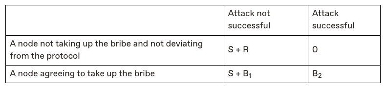
The post present a new model, the Corruption-Analysis model, in order to analyze slashing. They accompany the model with the following table that showcases the different outcomes of an attack in a protocol that does not have slashing:
Briefly, it shows that (in the bottom-left corner) failed attacks don't really have a cost as attackers keep their stake (S) and potentially get paid (B1) to do the attack. On the other hand it shows that (in the top-right corner) people will likely punish everyone in case of an attack by mass selling and taking the token price down to $0$ (an implied feature they call token toxicity).
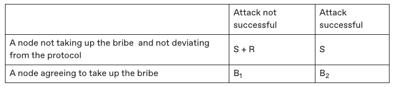
On the other hand, this is the table they show once slashing is integrated:
As one can see, the bottom-left corner and the top-right corner have changed: a failed attack now has a cost, and a successful attack almost doesn't have one anymore. Showing that slashing is strictly better than not slashing.
While this analysis is great to read, I'm not sure I fully agree with it. First, where did the "token toxicity" go in the case of a successful attack? I would argue that a successful attack would impact the protocol in similar ways. Perhaps not as intensely, as as soon as the attack is detected the attackers would lose their stake and not be able to perform another attack, but still this would show that the economic security of the network is not good enough and people would most likely lose their trust in the token.
Second, is the case where the attack was not successful really a net improvement? My view is that failed attacks generally happen due to accidents rather than legitimate attempts, as an attacker would most likely succeed if they had enough to perform an attack. And indeed, I believe all of the slashing events we've seen were all accidents, and no successful BFT attacks was ever witnessed (slashing or no slashing). (That being said, there are cases where an attacker might have difficulties properly isolating a victim's node, in which case it might be harder to always be successful at performing the attack. This really depends on the protocol and on the power of the adversary.)
In addition, attacks are all different. The question of who is targeted matters: if the victim reacts, how long does it take them to punish the attackers and publish the equivocation proofs? Does the protocol has a long-enough unstaking period to give the victim time to punish them? And if a third of the network is Byzantine, can they prevent the slashing from happening anyway by censoring transactions or something? Or worst case, can they kill the liveness of the network instead of getting slashed, punishing everyone and not just them (up until a hard fork occurs)?
Food for thought, but this shows that slashing is still quite hard to model. After all, it's a heuristic, and not a mechanism that you will find in any BFT protocol whitepaper. As such, it is part of the overall economic security of the deployed protocol and has to be measured via both its upsides and downsides.
I think a lot about how to express concepts and find good abstractions to communicate about proof systems. With good abstractions it's much easier to explain how proof systems work and how they differ as they then become more or less lego-constructions put up from the same building blocks.
For example, you can sort of make these generalization and explain most modern general-purpose ZKP systems with them:
They all use a polynomial commitment scheme (PCS). Thank humanity for that abstraction. The PCS is the core engine of any proof system as it dictates how to commit to vectors of values, how large the proofs will be, how heavy the work of the verifier will be, etc.
Their constraint systems are basically all acting on execution trace tables, where columns can be seen as registers in a CPU and the rows are the values in these registers at different moments in time. R1CS has a single column, both AIR and plonkish have as many columns as you want.
They all reduce these columns to polynomials, and then use the fact that for some polynomial $f$ that should vanish on some points ${w_0, w_1, \cdots}$ then we have that $f(x) = [(x - w_0)(x-w_1)\cdots] \cdot q(x)$ for some $q(x)$
They also all use the fact that proving that several identities are correct (e.g. $a_i = b_i$ for all $i$) is basically the same as proving that their random linear combination is the same (i.e. $\sum_i r_i (a_i - b_i) = 0$), which allows us to "compress" checks all over the place in these systems.
Knowing these 4-5 points will get you a very long way. For example, you should be able to quickly understand how STARKs work.
Having said that, I more recently noticed another pattern that is used all over the place by all these proof systems, yet is never really abstracted away, the interactive arithmetization pattern (for lack of a better name). Using this concept, you can pretty much see AIR, Plonkish, and a number of protocols in the same way: they're basically constraint systems that are iteratively built using challenges from a verifier.
Thinking about it this way, the difference between STARK's AIR and Plonks' plonkish arithmetization is now that one (Plonk) has fixed columns that can be preprocessed and the other doesn't. The permutation of Plonk is now nothing special, the write-once memory of Cairo is nothing special as well, they're both interactive arithmetizations.
Let's look at plonk as a table, where the left table is the one that is fixed at compilation time, and the right one is the execution trace that is computed at runtime when a prover runs the program it wants to prove:
One can see the permutation argument of plonk as an extra circuit, that requires 1) the first circuit to be ran and 2) a challenge from the verifier, in order to be secure.
As a diagram, it would look like this:
Now, one could see the write-once memory primitive of Cairo in the same way (which I explained here), or the lookup arguments of a number of proof systems in the same way.
For example, the log-derivative lookup argument used in protostar (and in most protocols nowadays) looks like this. Notice that:
in step 4 the execution trace of the main circuit is sent
in step 6 the verifier sends a challenge back
and in step 7 the prover sends the execution trace of the second circuit (that implements a lookup circuit) using the challenge
As such, the point I really want to make is that a number of ZKP primitives and interaction steps can be seen as an interactive process to construct a super constraint system from a number of successive constraint system iterated on top of each other. Where constraint system means "optionally some new fixed columns, some new runtime columns, and some constraints on all the tables including previous tables". That's it.
Perhaps we should call these iterative constraint systems.
In this episode, David Wong introduces Ethereum and explains its account-based model and the concept of smart contracts. He compares Ethereum to Bitcoin and highlights the advantages of Ethereum's more expressive programming capabilities. He also discusses the execution of transactions and the role of the Ethereum network in maintaining the state of smart contracts.